Binary Trees

A look at binary trees

Binary trees are a fundamental data structure in computer science and their applications stretch beyond computer science into many domains. They can be found in binary search trees, binary heaps, syntax trees, hash trees and more. The first thing that comes to mind for many of us when we hear the word ‘binary tree’ is binary search tree. The binary search tree is a very popular implementation of a binary tree that I will be covering later on in this post. I wanted to cover regular binary trees first because it’s important to understand their generic properties and aspects before we dive into something more specific. I’ll be covering the different types of binary trees, binary tree traversal, and a few other pertinent details, so without further ado let’s dive in!

Let’s start by looking at the “tree” in binary tree. A tree is a data structure that has a root, which is a node, and each node has 0 or more children. Each child of the root is itself a tree and follows the definition we just listed. Essentially, every single node in a tree is a tree itself. A binary search tree is a tree where for each node in this tree, that node can have 0, 1, or 2 children. The name binary comes from the fact that each node can have 2 children, a ternary tree for example has nodes with up to 3 children. These children are called the left child and the right child, and each node has pointers to these children. We sometimes also maintain a parent pointer in a node, where the parent is the node of which I am a child of, though this is less common. It’s important to note that 2 is a maximum bound on the number of children, certain nodes may have 0 children, these are called leaf nodes. Leaf nodes are nodes without children, which makes sense because like a leaf on a tree we cannot branch out further once we reach a leaf node. The defining mark of a leaf node is that their pointers to the left and right child are null.

Height: The height of a binary tree is the longest path from the root to the bottom of the tree. Depth: The depth of a node in a binary tree is the number of nodes from the root to the node, the depth of the root is 0; Level: The level of a binary tree is all the nodes that are found at a certain height. So, the root is at level 0, we can have 2 nodes at level 1, 4 nodes at level 2 etc…

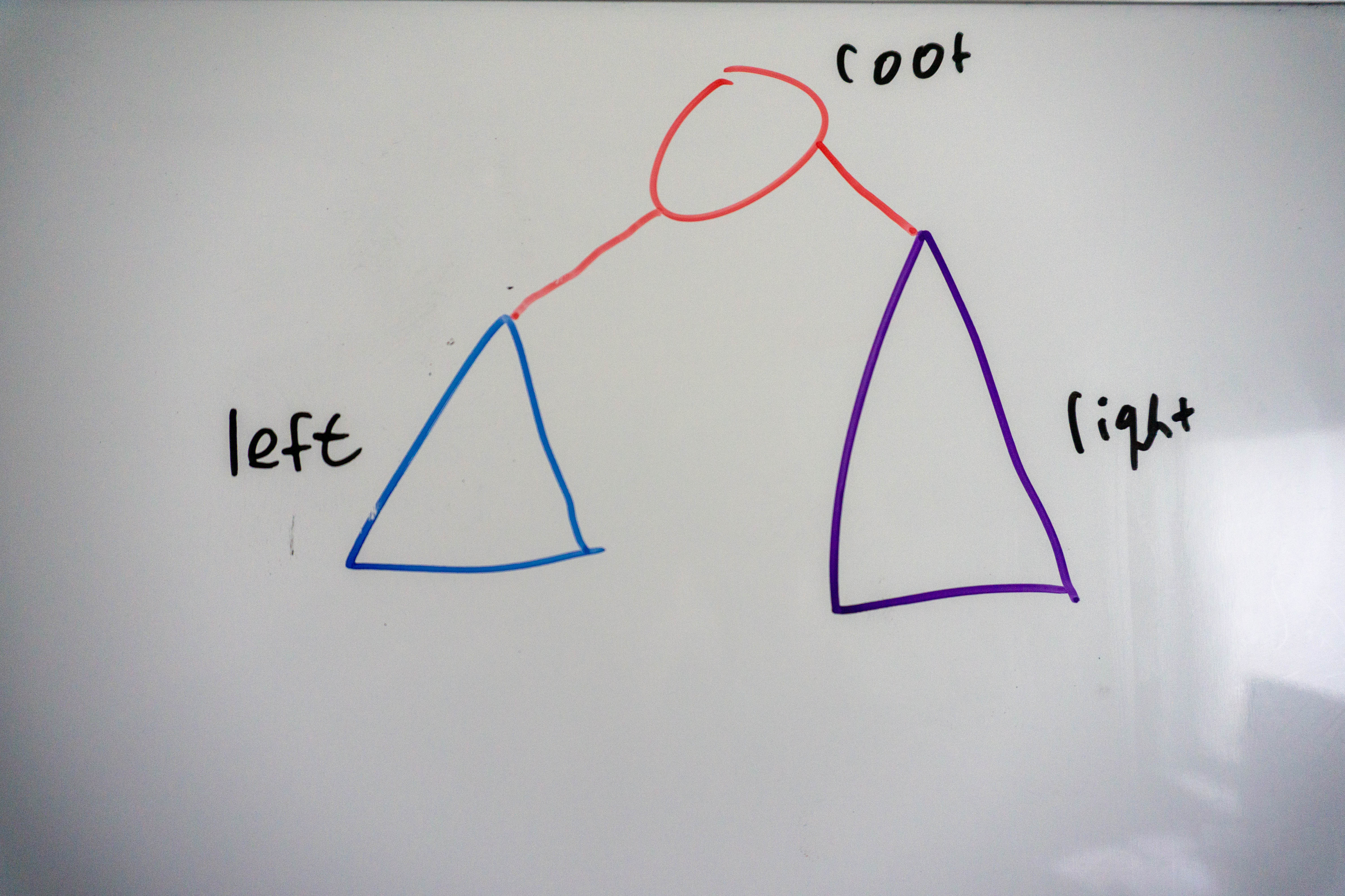The blue and purple triangles represent binary trees. These can be the same size, or they may differ

Let’s take a look at some of the binary trees we can make with 1,2, or 3 nodes:

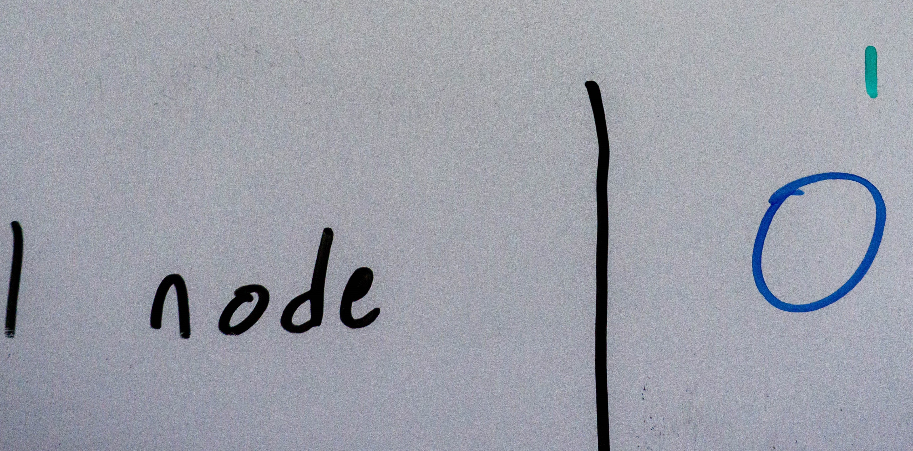A binary tree with 1 node has 1 possible configuration, this binary tree has height 1.

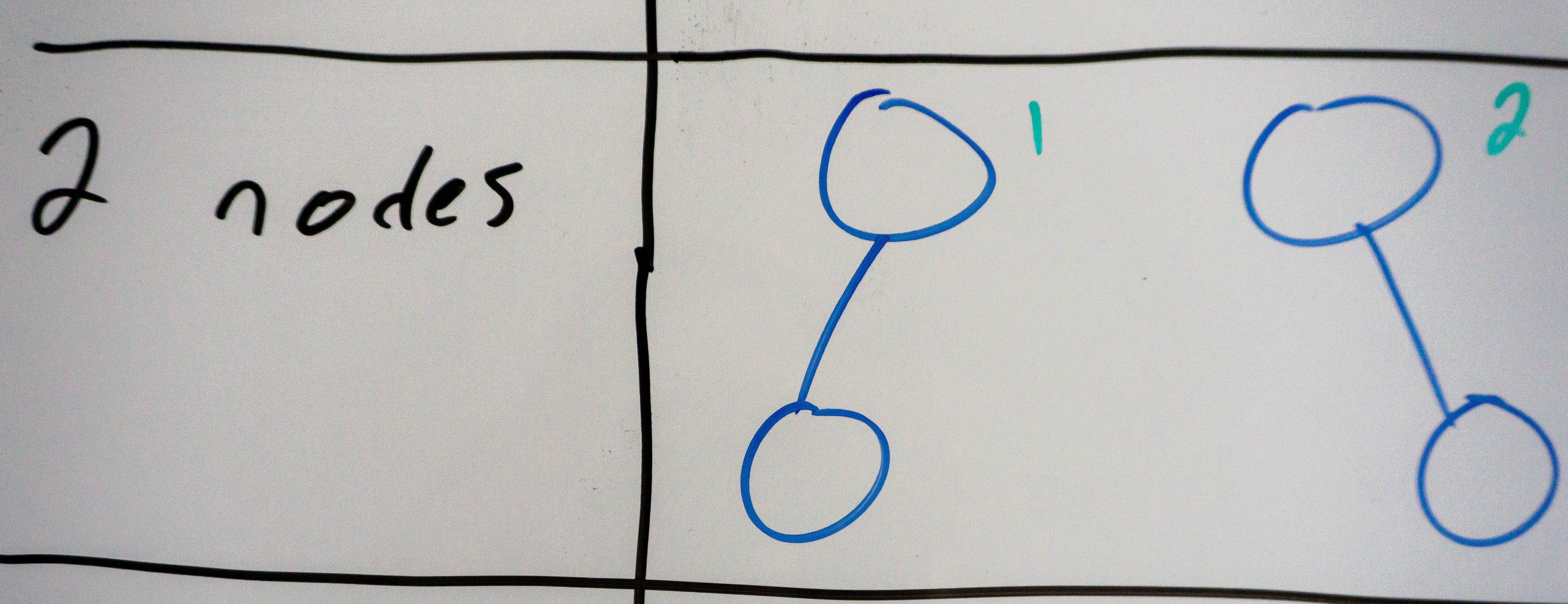A binary tree with 2 nodes has 2 possible configurations, with a height of 2.

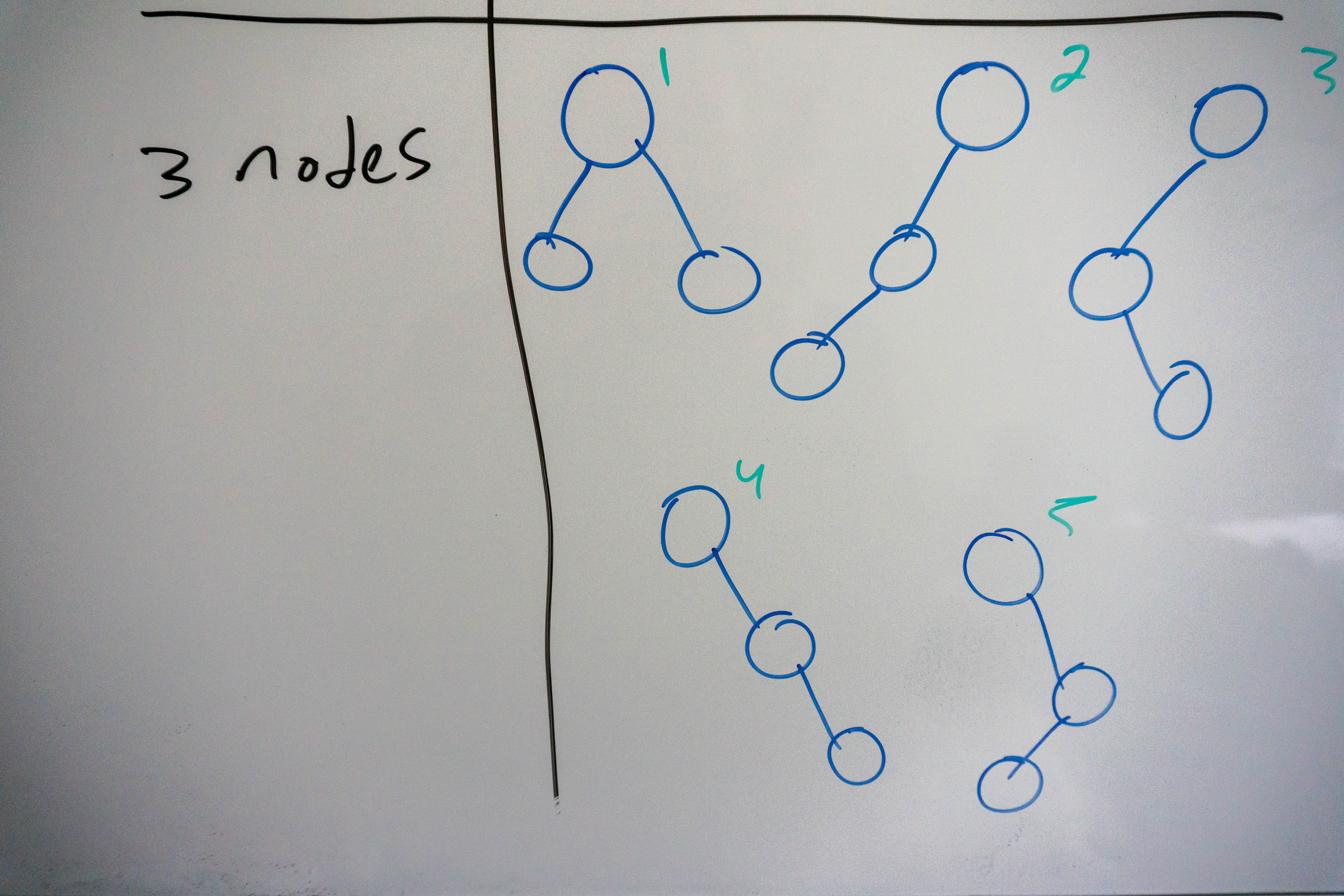A binary tree with 3 nodes has 5 possible configurations, with a maximum height of 3.

Balanced Binary Trees

A binary tree is considered balanced when the height of the left and right subtrees differ by no more then 1. This must be true for every node in the tree. Why do we concern ourselves with the balance of the tree? For binary search trees an unbalanced tree can leave us with a worst-case time complexity of O(n) for search, which is not good since binary search trees are supposed to give us O(log n) search! I’ll talk about binary search trees a little later, just remember that a balanced binary tree is one in which the height of the left and right subtrees differ in height by no more than 1.

Types of binary trees

There are 3 sub-types of binary trees we will concern ourselves with here, these are : complete binary trees, full binary trees and perfect binary trees.

Complete binary trees

A complete binary tree is a binary tree in which each level of the binary tree is filled, except for possibly the last level, which if partially filled, is filled from left to right. In other words, each node on every level before the last level has 2 children. The last level can be partially filled, but any nodes must be inserted from left to right, here is an example: 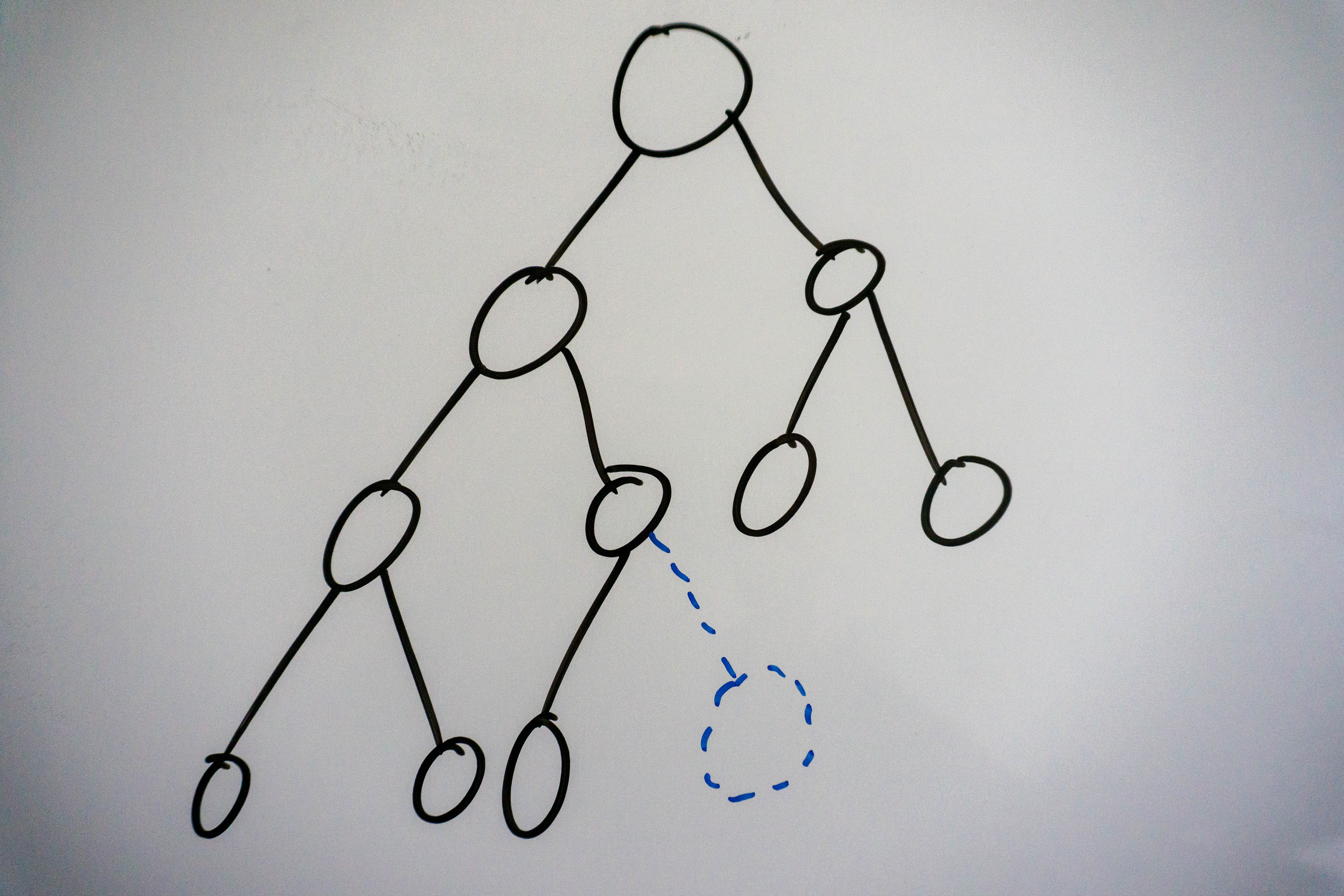The dashed blue node shows where the next node would go in our tree.

Full binary trees

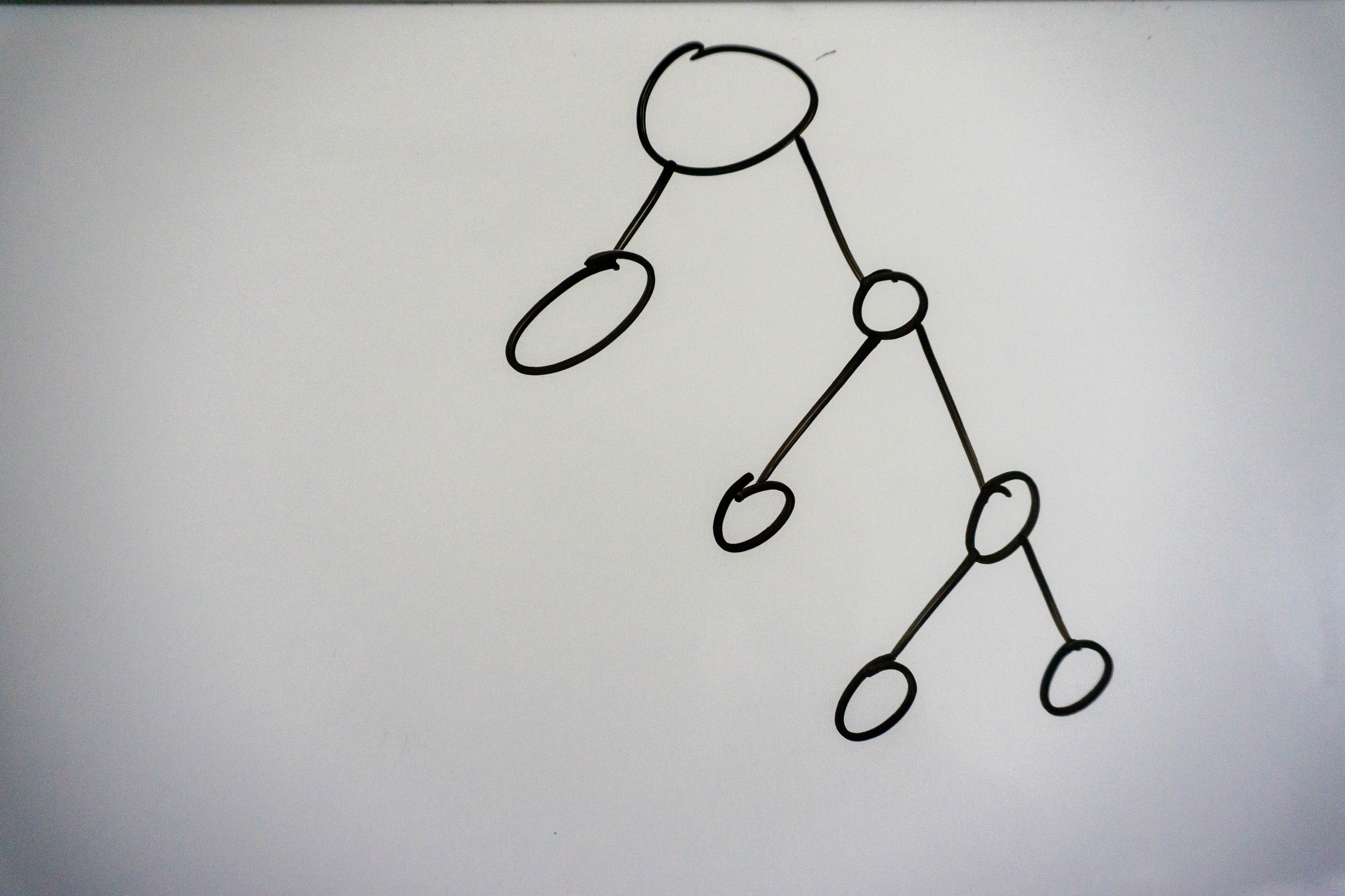
A full binary tree is a binary tree where each node has 0 or 2 children, there can be no nodes with 1 child, here’s an example:

Perfect binary trees

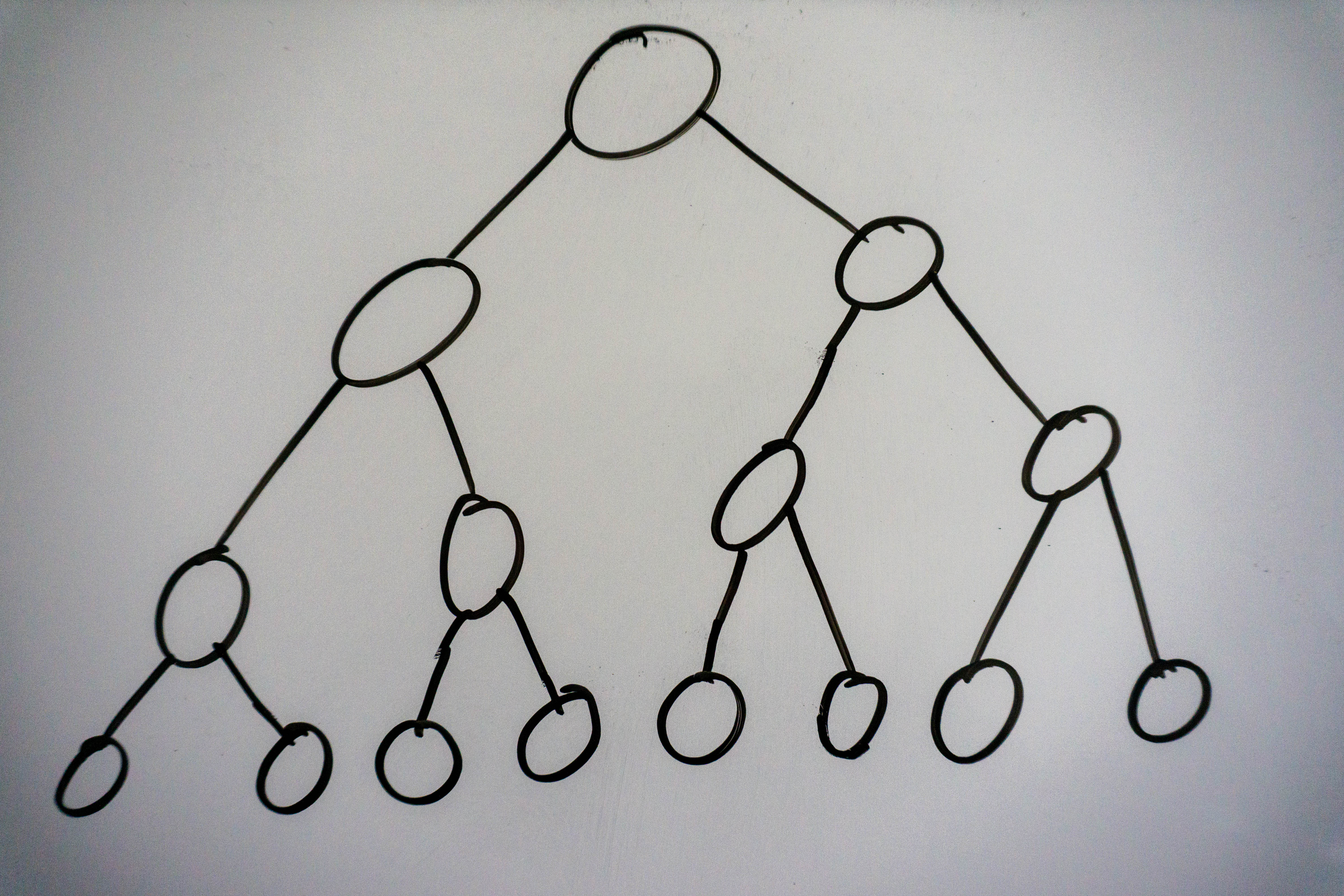
A perfect binary tree is a binary tree that is both complete and full. This type of tree is rare and doesn’t come up too often, but it’s good to know it exists. Below is an example:

Binary Tree Traversal

There a 3 main types of binary tree traversals, these are : pre-order, in-order, and post-order traversal. In pre-order traversal we visit the root first, then the left subtree, and finally the right subtree. In-order traversal has us visiting the left subtree, the root, and finally the right subtree. A post-order traversal visits the root last, visiting the left subtree first, then the right subtree, and finally the root. Let’s see in what order we visit the nodes for the tree below:

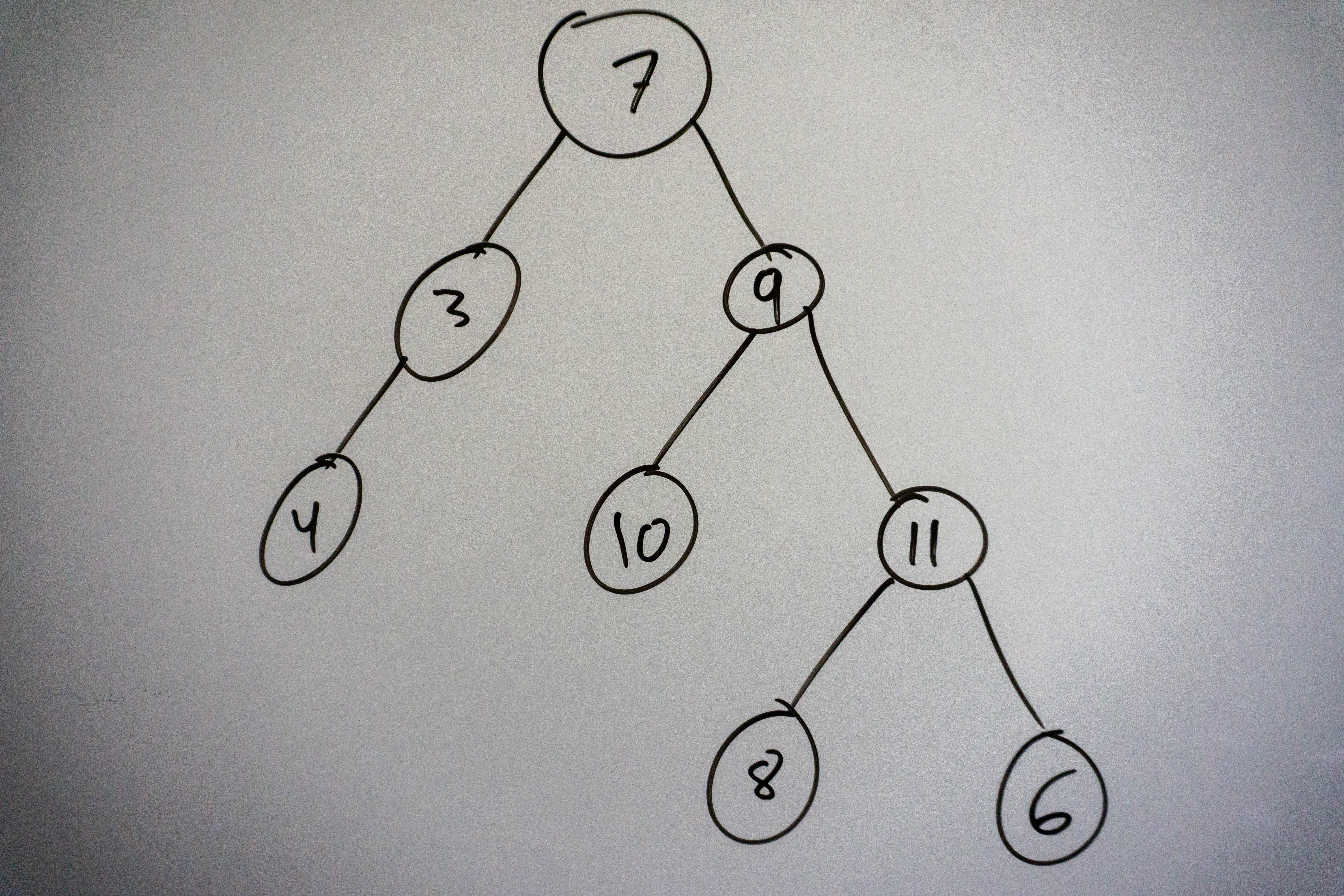
Pre-order: 7 -> 3 -> 4 -> 9 -> 10 -> 11 -> 8 -> 6

In-order: 4 -> 3 -> 7 -> 10 -> 9 -> 8 -> 11 -> 6

Post-order: 4 -> 3 -> 10 -> 8 -> 6 -> 11 -> 9 -> 7

Binary Search Trees

Binary Search trees are a special case of binary trees where all nodes smaller than the root are on the left, and all nodes bigger than the root on the root. If we allow duplicates the common convention is to add them to the left of the root, but you could add them on the right if you wanted to. Why is this type of tree so powerful? It allows us to search in O(log n) time when the tree is balanced! The main idea behind binary search is that we compare the value we are looking for with the root. If the value is less than the root we go left, and search that subtree, if the value is larger we go right and search that subtree. The key principle here is that each time we go left or right, we reduce our search space in half. After the first comparison we are left with roughly 1/2 the nodes to look through. After the second comparison we are left with roughly 1/4 of the nodes to search through. This continues until we either find the node we are looking for or reach the end of the tree, in which case our value is not in the tree. So why did I specify that it’s O(log n) if the tree is balanced? Consider the worst case where the height of the tree is n, in which case our tree can look like this:

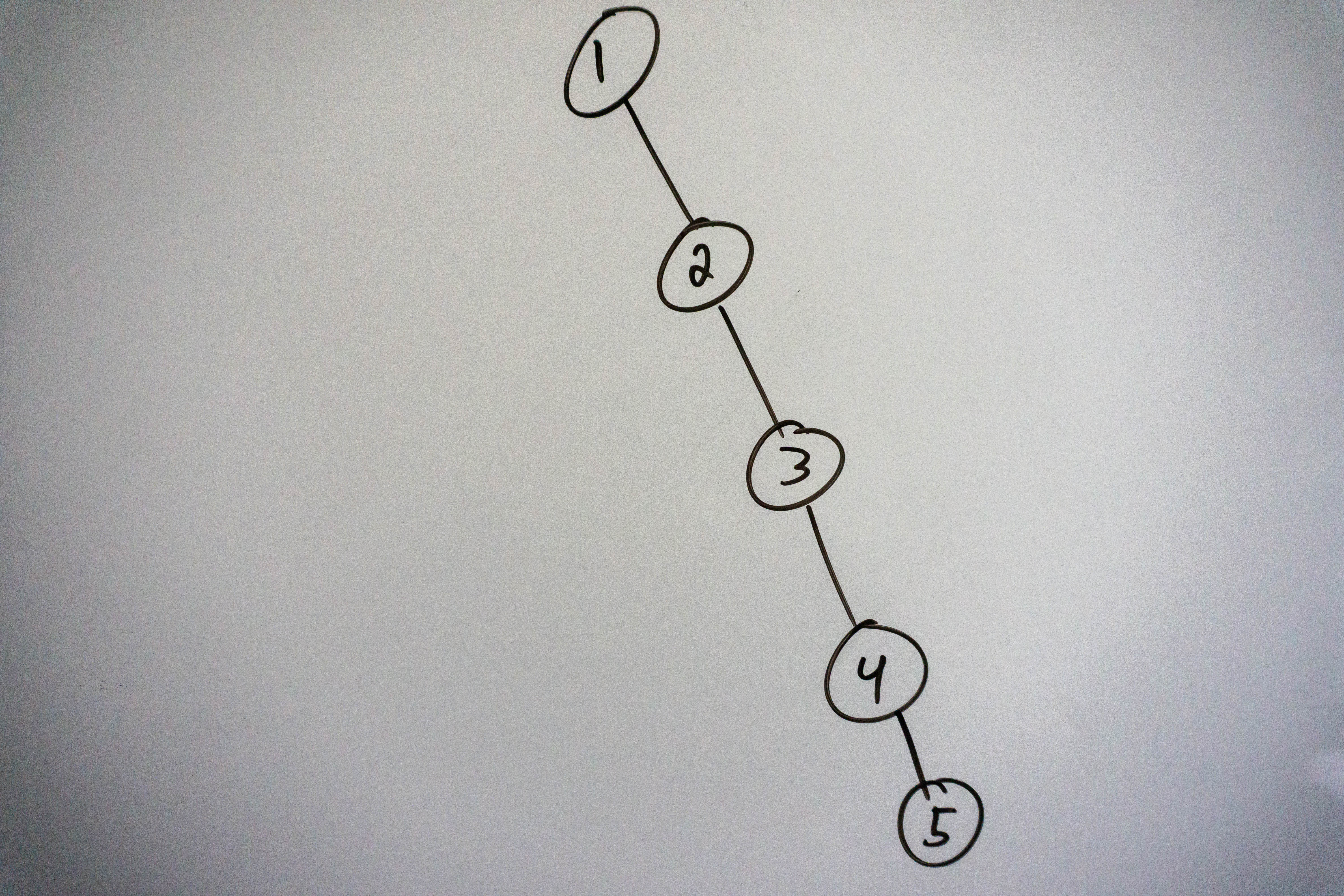
In that case our search takes O(n), which is no better than just searching through an array normally. This happens because search time correlates directly with the height of our tree. The time complexity of our search is in fact O(h), where h is the height of our tree. For the case where our tree is balanced the height is roughly log n, in the worst unbalanced case, it can grow all the way to n, which is why the time complexity becomes O(n).

Self Balancing Binary Trees and Final Thoughts

Before we wrap things up, I quickly wanted to touch on two types of self balancing binary search trees called AVL Trees and Red Black Trees. Without going into specifics, these two types of binary search trees contain algorithms to automatically rebalance the tree when it becomes unbalanced. Therefore, when we use a self balancing tree we can avoid the problem where we have a worst-case height of O(n), and guarantee our height will be roughly equal to O(log n). There exist other types of self balancing binary search trees, these 2 are the ones I see come up most often however. Don’t worry too much about their specific implementation, just know that they exist.

That concludes this post on binary trees, I hope you’ve found it helpful. It’s very important to be comfortable with binary trees, I recommend implementing a binary tree and binary search tree in your language of choice to deepen your understanding of these data structures. As always, stay tuned for more content and have a good day!